Understanding Neural Networks from Geometric Perspective

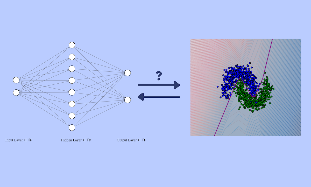
If you’ve worked with neural networks, you’re likely familiar with how they function—at least the forward pass (if not, don’t worry; I’ll summarize it in the next section). At their core, neural networks rely on matrix multiplication, addition, and element-wise operations. However, developing an intuitive understanding of how they recognize patterns is just as important.

For very deep neural networks, understanding their inner workings can be challenging. However, with shallow and low-dimensional networks, we can still analyze their behavior to some extent. In this blog, I will explain how neural networks perform pattern recognition from a geometric perspective. By visualizing how neural network weights interact with input data, we can gain insights into their decision-making process. I will illustrate this using various visualizations in coordinate space, primarily in 2D.

Our focus will be on understanding how neural networks work rather than how they are trained. Topics such as backpropagation and optimization algorithms will NOT be covered here.

The code used here for experiments & generating visualizations can be found here .

Single Neuron

Definition

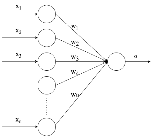
Let’s say each sample in input data consist of $N$ features: $X={x_1, x_2, x_3, …, x_N}$. Simple put, $X$ contains $N$ numerical values, which could represent anything from pixel intensities in an image to parameters like height, weight in tabular data. The output of the single neuron is defined as follows:

$$ o = \sigma (x_1 w_1 + x_2 w_2 + x3 w_3 + … + x_n w_n + b_1) $$

Here the $W={w_1, w_2, w_3, …, w_n}$ represents weight associated with each input element $x$ and $\sigma$ is an activation function. The term $b_1$ is the bias(more on activation function and bias later). The neuron’s activation is determined based on whether its output is positive or negative—though the actual value also plays a role.

Geometric Meaning

If closely examine the equation and recall your lienar algebra (or even physics) classes, you will notice that it resemebles the to dot product equation. Let’s first formally define everything in the vector form.

Let $X = [x_1, x_2, x_3, …, x_N]$ be the input data vector and $W=[w_1, w_2, w_3, …, w_N]$ be the weight vector. Then the output of the single neuron is defined as:

$$ o = \sigma( X \cdot W) $$

Let’s temporarily ignore the activation function and focus on the dot product. Geometrically, the dot product measures the angle between two vectors—in other words, how similar they are. If both vectors are normalized, a dot product value of 1 means they point in the same direction, a value of 0 means they are perpendicular, and a negative value indicates they point in opposite directions.

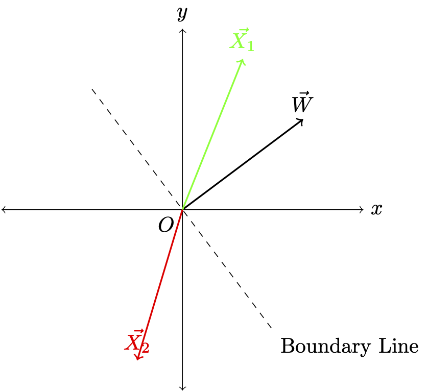
This means that if the input data vector forms an angle of less than $90\degree$ with the weight vector, the output will be positive. This is a crucial observation because a line perpendicular to the weight vector represents the set of vectors where the dot product output is zero. This perpendicular line acts as a decision boundary for the neuron. If a vector lies on the same side of this boundary as the weight vector, the output will be positive; otherwise, it will be negative. The output value also depends on how close the input data vector is to the weight vector. By adjusting the weight vector, you can modify the slope of the boundary line.

Role of Bias

You may have noticed that the boundary line passes through the origin and remains fixed there. While you can change its slope, you cannot shift it in space. To introduce this flexibility, we can translate the weight vector by adding a scalar value. If you guessed correctly, this scalar value is the bias $b_1$ ​that we introduced earlier in the equation. With this, we now have the flexibility to adjust both the slope ($m$) and the intercept ($c$) of the boundary line.

Visualizing Boundary line

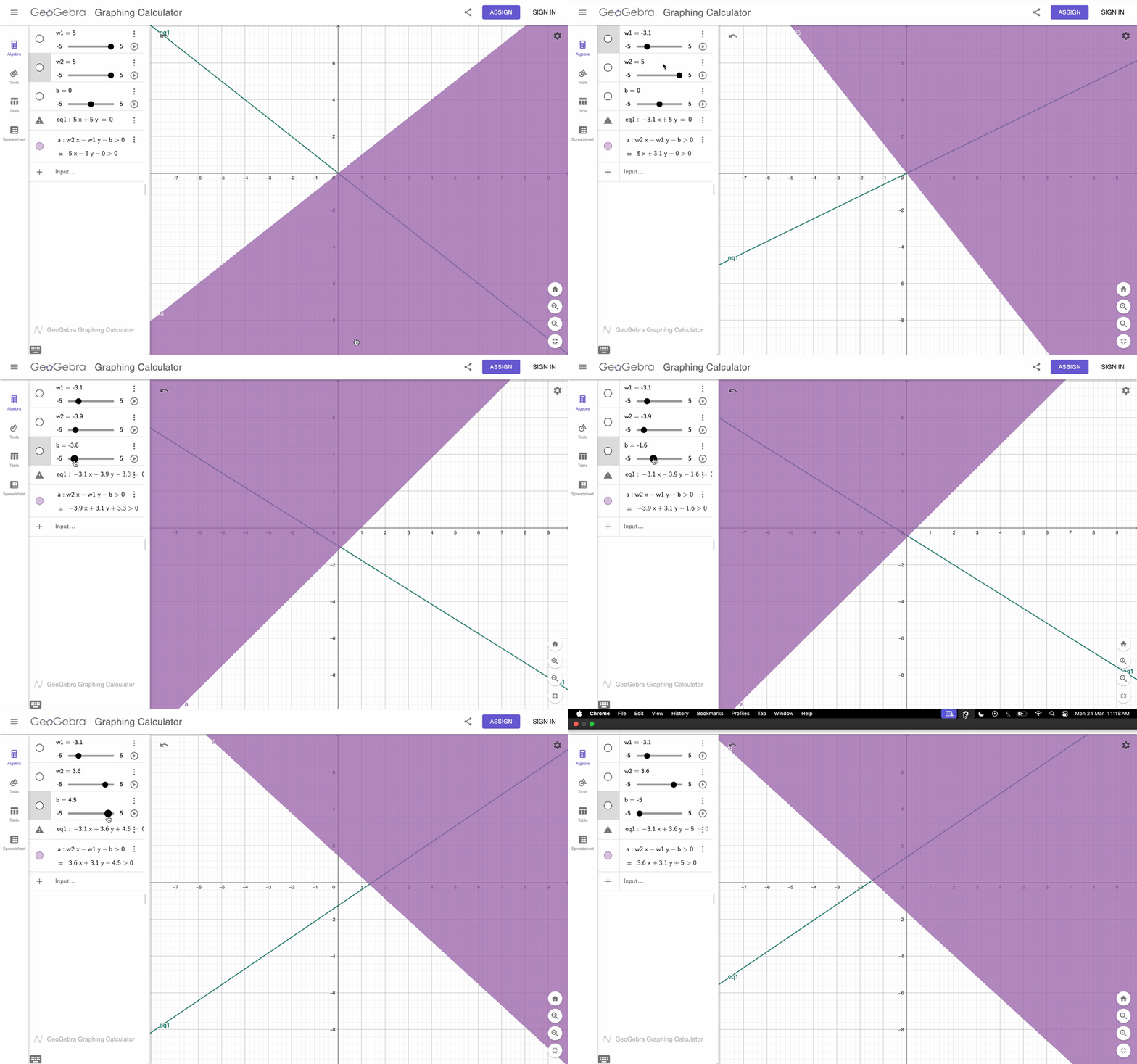
For a two-dimensional example, we can visualize how the boundary line shifts by adjusting the weight vector and bias, plotting it in Cartesian space.

Role of Activation Function

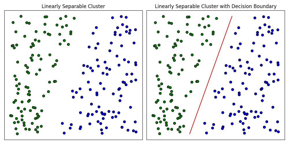
If I showed you the above plot and asked you to separate the two color-coded data points, you could easily do so by drawing a straight line that divides them. In Euclidean geometry, such data is called linearly separable if at least one line exists that can separate the two sets of points.

In machine learning terms, this represents a classification problem in $2D$ space. The neuron learns the $2D$ weight vector $W$ and bias $B$, which together define a boundary line that separates the two sets of points. (Note that how the neuron learns to do this is beyond the scope of this post.)

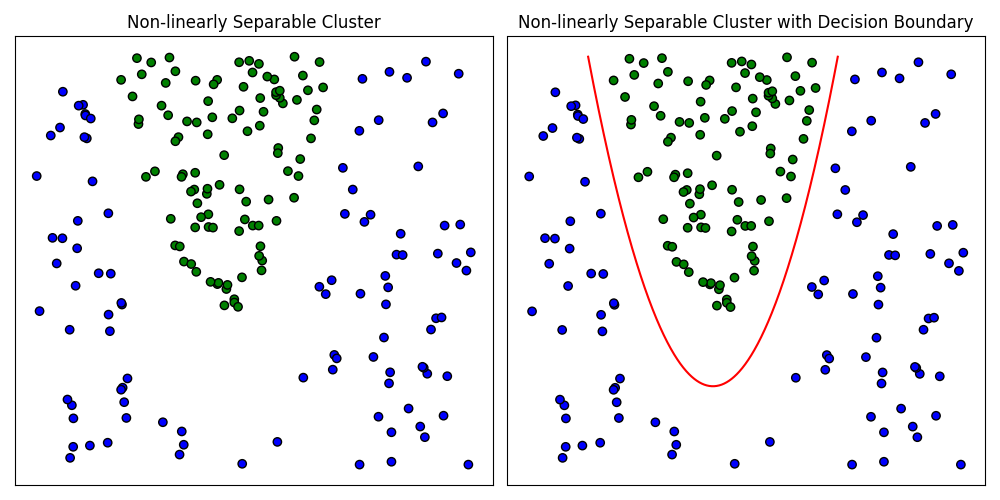
Now, if I showed you the same plot and asked you to separate the points, you might struggle to do so with a straight line. Instead, you would likely draw a curved boundary, as shown in the second image. These points are not linearly separable, which is why we need to introduce some form of non-linearity into the dot product equation. This is where activation functions come in.

An activation function is any non-linear function applied to the dot product. While there are certain mathematical properties that make activation functions more effective for training, their primary role is to introduce non-linearity.

If you’ve studied other machine learning algorithms, you may notice that using the sigmoid function as an activation function makes a single neuron functionally equivalent to logistic regression.

So far, we have mostly understood a neuron’s function from the perspective of a $2D$ input space. However, we can generalize this concept to an $N$-dimensional space as well.

In higher dimensions, the equation represents the distance of a point $P$ from a hyperplane, which is defined by the directional vector $\vec{W}$ and the offset $b$. You can find the derivation for this using linear algebra here.

Neural Network

A single neuron alone is limited to performing linear classification. Even with an activation function, its flexibility remains constrained. However, when multiple neurons are stacked within a single layer, the model can learn multiple decision boundaries for the same input data. Adding another layer further enhances learning, enabling the network to capture more complex patterns and relationships.

Toy Example

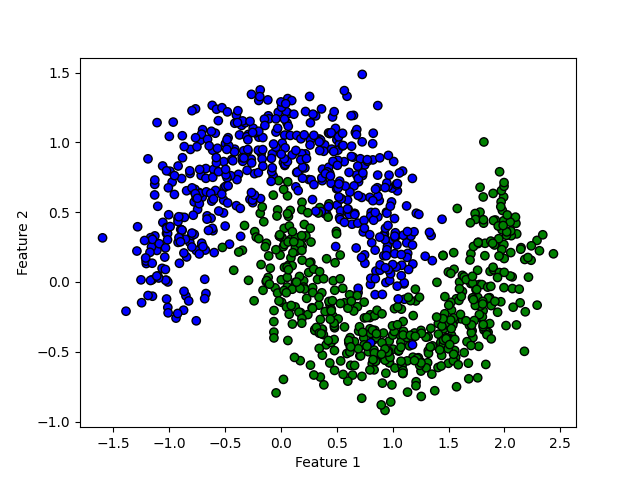
To understand neural networks, we will consider a simple toy example of 2D classification, as shown in the figure above. The data is clearly not linearly separable and is more complex than the previous example. To tackle this, we will use a neural network with a single hidden layer containing 8 neurons, followed by an output layer with 2 neurons.

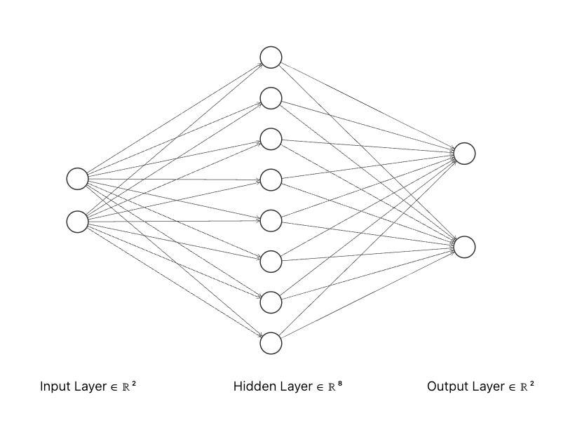
You could use single neuron for the output if using torch.nn.BCEWithLogitsLoss, but I am keeping it more generalized by using torch.nn.CrossEntropyLoss. Additionally, I am using Relu activation, Adam optimizer wuth a fixed learning rate of 0.01 and 100 epochs for training.

Visualizing hidden layers’ boundaries

We wil define the hidden layer’s weight matrix $W$ of size $[8, 2]$ as a collection of vectors $[w_0, w_1, …, w_7]$ each havinga dimensionality $2$. In other words, each $w_i$ is a row vector of weight matrix $W$.

Let’s visualize the decision boundaries created by each of these weight vectors without, both before and after applying the activation function, once training is complete.

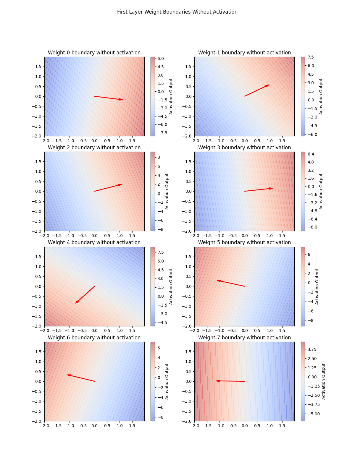
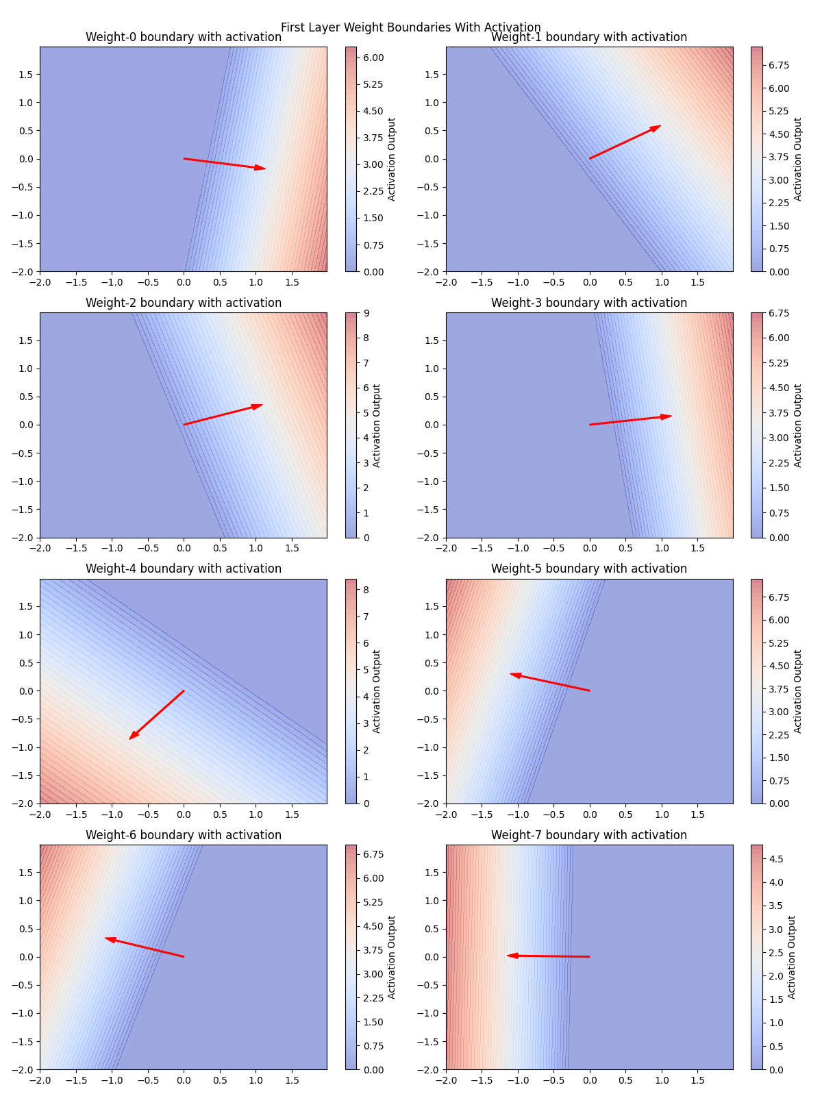
If you’re wondering how these boundary visualizations are created, let me explain. We generate a 2$D$ grid of points (xy coordinates), where each point represents an input to the neural network. These points are then fed into the network, and we store the hidden layer’s output. The results are then displayed as a heatmap, allowing us to analyze how each neuron responds to all possible input points, not just those in the dataset.

As expected from the mathematical derivation, the boundary is clearly perpendicular to the weight vector. Although we have multiple boundaries here, they are independent at this stage and do not contribute to learning non-linear patterns. However, the next layer can utilize these linear boundaries to construct more complex decision regions.

Visualizing output layer’s boundary

Now, let’s visualize the output layer of this neural network.

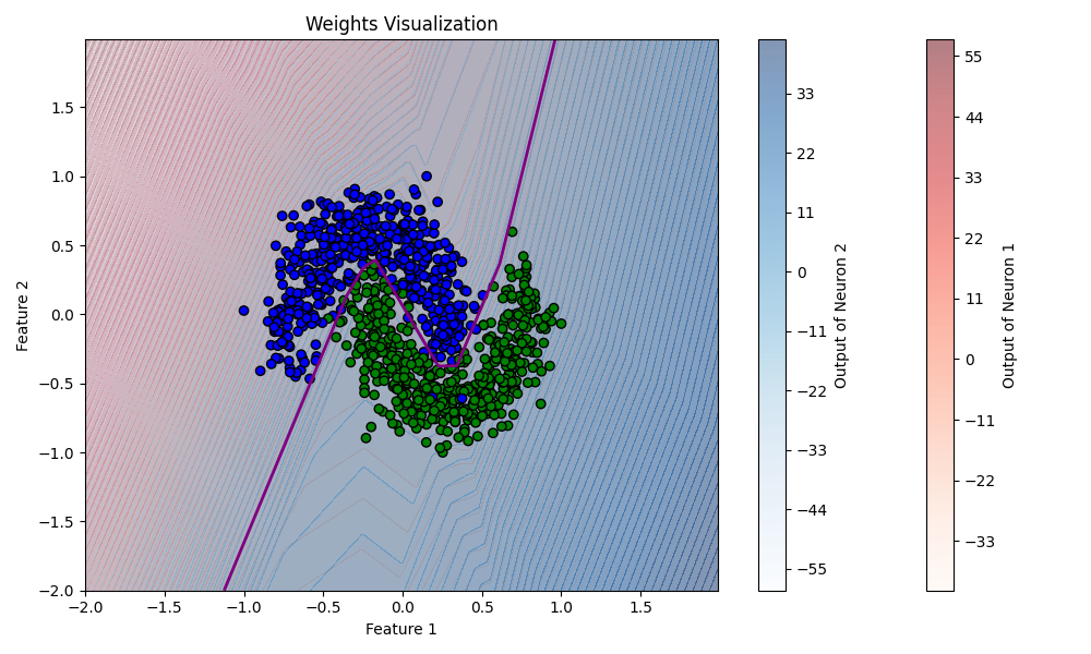
Classification is determined by comparing the output values predicted by the first and second neurons in the output layer. If the first neuron’s score is higher than the second neuron’s, the input is classified as Class 1; otherwise, it is classified as Class 2.

The purple boundary represents the decision boundary where both neurons output the same value. Additionally, you can observe how the red and blue colors fade as they approach the boundary, indicating that the output neuron values are decreasing. This suggests that the network is less confident about the classification near the boundary.

---

There’s another interesting observation about the boundary line—can you spot it?

The boundary line is indeed non-linear now, adapting to the distribution of both classes. However, it is piecewise linear—meaning that this non-linear boundary is composed of multiple linear segments with different slopes, connected together.

This happens because the output layer utilizes the boundary lines (shown in Figures 7 & 8) created by the hidden layer’s neurons to form the final decision boundary. Keep in mind that the output layer also has its own weights and biases, so the final boundary line is essentially a weighted summation of the previous boundary lines.

This gives us an intuitive understanding that while solving a classification problem, each hidden layer neuron is learning a specific type of boundary. As we go deeper, these boundaries are combined to form more complex decision boundaries.

These intermediate boundaries may or may not have a direct interpretation with respect to the input data points in the same space. However, by the time we reach the output layer, we can clearly visualize the final complex boundary that effectively separates the input data points.

This is also why we typically use the outputs from the hidden layer just before the output layer as an embedding or representation vector in networks like ResNet. This layer contains the most useful information for defining decision boundaries that effectively separate data points into different classes.

Remember, we were able to analyze this because our dataset was 2$D$, but in real-world scenarios, datasets are rarely this simple. For example, an RGB image with a resolution of 64×64 pixels would have a dimensionality of 64×64×3 = 12,288, making it extremely challenging to visualize decision boundaries in the same way.

However, the same concept applies in higher dimensions, where the boundary line is replaced by a hyperplane that separates data points in a multi-dimensional space.

Visualizing boundary during training

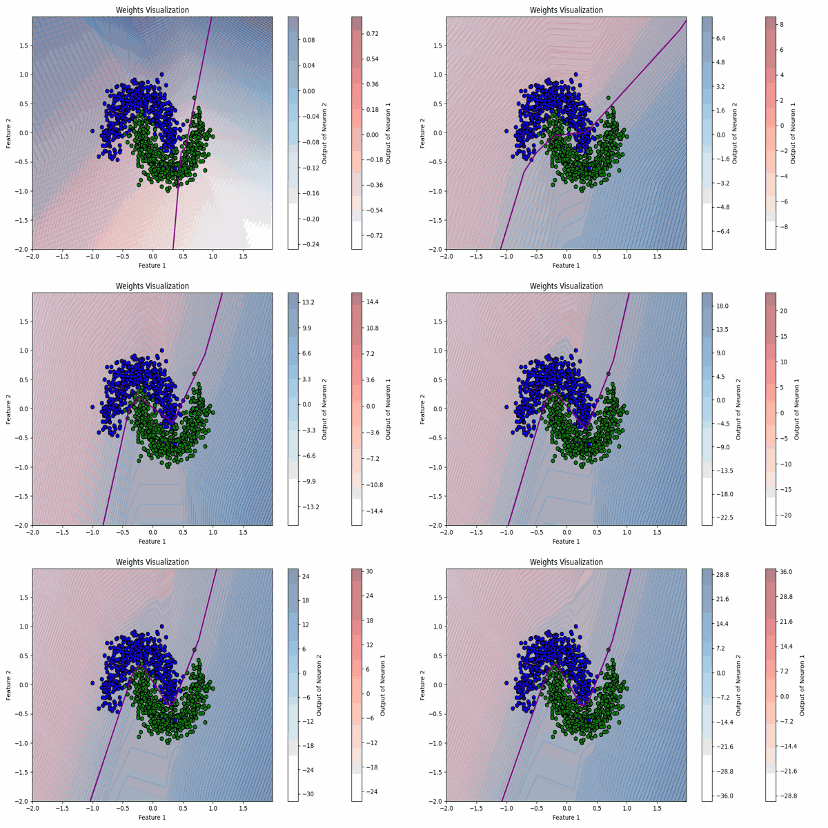
Another interesting visualization is observing how the boundary line from the output layer evolves as the neural network progresses through training. This allows us to see how the network gradually adjusts its decision boundary, refining it step by step to better separate the data points.

Key Takeaways

• The weight matrix of each hidden layer in a neural network can be broken down into multiple weight vectors, each corresponding to a neuron.
• Each weight vector represents a boundary hyperplane, where the output is positive if the input data lies on the same side as the weight vector and negative otherwise. The activation function helps transform this linear boundary into a non-linear one.
• The hidden layer takes the boundary hyperplanes from the previous layer and combines them to form even more complex hyperplanes.
• The output layer constructs the final hyperplane in the D-dimensional input space, effectively separating data points based on their classes.

Going Further

• We only used the ReLU activation function here. Can you think about what would happen if we had used sigmoid or tanh instead? How would it affect the boundary line in this example?
• What if we added one more hidden layer? Would it help in learning a better boundary? How would it impact the network’s ability to separate the data?

Feel free to reproduce my experiments using the code here or tweak it to generate new visualizations for the above questions.